As in Goldvarb, it is always a good idea to cross-tabulate your data by some of the factors of interest, before performing any kind of multiple regression. By calling the R function xtabs, Rbrul can create two types of crosstabs, one showing "counts" (the total number of tokens) in each cell, and the other showing the average value of the response (dependent) variable. For a continuous (numeric) response variable, the mean is shown for each cell; for a factor, we see the proportion of the application value(s). (If an independent variable is numeric, or is a factor with many values, a crosstab will still be generated, but the output may not be very useful. Display such variables in rows, not columns!)
Since we have not chosen a response variable yet, we will be prompted to do so, and to pick the application value(s) in the case of a factor. In this case, we will choose r for the response and 1 for the application value, and so the crosstab will show the proportion of (r-1), that is, the proportion of articulated (non-vocalized) /r/ for each cell.
The example below cross-tabulates by word in the columns and store in the rows. The function can also show a third dimension, by showing multiple "pages" of two-dimensional cross-tabulations. Here we omit the third dimension, but show both counts and proportions of the response. We begin by entering 4 for crosstabs from the Main Menu:
Cross-tab: factor for columns? (1-r 2-store 3-emphasis 4-word)
1: 4
Cross-tab: factor for rows? (1-r 2-store 3-emphasis Enter-none)
1: 2
Cross-tab: factor for 'pages'? (1-r 3-emphasis Enter-none)
1: [Enter]
Cross-tab: variable for cells? (1-response proportion/mean Enter-counts)
1: [Enter]
counts
word
store fouRth flooR total
Klein's 112 104 216
Macy's 175 161 336
Saks 95 82 177
total 382 347 729
...
Cross-tab: variable for cells? (1-response proportion/mean Enter-counts)
1: 1
Choose response (dependent variable) by number (1-r 2-store 3-emphasis 4-word)
1: 1
Type of response? (1-continuous Enter-binary)
1: [Enter]
Choose application value(s) by number? (1-0 2-1)
1: 2
proportion of r = 1
word
store fouRth flooR total
Klein's 0.080 0.115 0.097
Macy's 0.263 0.491 0.372
Saks 0.337 0.634 0.475
total 0.228 0.412 0.316
This method, of selecting variables from numbered lists, and choosing between options (often with Enter as a default), is used throughout Rbrul. We also note that the proportions in the second crosstab are displayed to three decimal places. This is a default, which can be changed under settings.
The first crosstab allows us to see that this dataset is well-balanced across word (unsurprisingly, given the methodology), and fairly evenly distributed across store as well. This means that an inspection of the column and row (marginal) proportions would be meaningful; these could be obtained by selecting a one-dimensional crosstab.
The second crosstab shows the cell proportions, where we observe the well-known regular patterns: increased use of (r-1) going up the social scale from Klein's to Macy's to Saks, and more (r-1) in stressed, word-final floor than in fourth.
We also observe evidence of an interaction here, as social stratification seems to be somewhat greater for the word floor (log-odds range 2.59) than for the word fourth (range 1.77). There are several ways to handle interactions in Rbrul. As in Goldvarb, users can 'manually' split the data and run parallel regressions, or create an interaction factor group (see Paolillo 2002 for more on these methods). This is done using exclude and cross in the Adjusting Menu. Alternatively, there is the test interactions option in the Modeling Menu. Here, for simplicity, we will continue towards a multiple regression analysis, setting aside the issue of factor interactions.
2. Modeling
Choosing 5 from the Main Menu opens the Modeling Menu, which contains several similar functions for performing regression analysis (one-level, step-up, step-down, and step-up/step-down). There is also an option to change various settings, mainly affecting the operation and output of the modeling functions. Before we can use any of the modeling functions, we have to choose which variables will be considered as candidates for the model, so we select 1-choose variables.
2.1 Choose Variables
This function allows us to decide which variables will be considered for inclusion in a regression model, and in what way. First it asks for a single response (dependent) variable, and determines its type (binary or continuous). Then it asks for a list of the predictor variables (explanatory, or independent variables), and asks us to specify their type: whether they are categorical or continuous, and whether they should be treated as fixed or random effects.
If the response is binary, it sets Rbrul up to perform logistic regression; otherwise, linear regression. If random effects are included, then mixed models will be fit using the glmer function; if not, traditional linear or logistic models are fit with glm.
In general, if your data includes a large number of potential independent variables, it is not always the best idea to throw them all into a stepwise regression. This is especially true when some of the variables are correlated. In the simplified department store data, there are only three independent variables, and we have every reason to consider them all from the outset. All variables are categorical (factors), and there is no candidate for a random effect, when we remember that each observation at a given level ofstore, emphasis, and word was obtained from a different person. (There are 729 observations from 264 individuals; I am emphasizing this because typical sociolinguistic interview data has a very different structure, with many tokens from each speaker.)
We enter 1 from the Modeling Menu and proceed to choose variables as follows, again selecting the value 1 (the presence of /r/) as the application value for the response, and pressing Enter to skip those questions (continuous variable, random effect) that do not apply to this data:
Choose response (dependent variable) by number (1-r 2-store 3-emphasis 4-word)
1: 1
Type of response? (1-continuous Enter-binary)
1: [Enter]
Choose application value(s) by number? (1-0 2-1)
1: 2
Choose predictors (independent variables) by number (2-store 3-emphasis 4-word)
1: 2
2: 3
3: 4
Are any predictors continuous? (2-store 3-emphasis 4-word Enter-none)
1: [Enter]
Any grouping factors (random effects)? (2-store 3-emphasis 4-word Enter-none)
1: [Enter]
No model loaded.
Current variables are:
response.binary: r
fixed.categorical: store emphasis word
We see at the bottom of this output that we have still not loaded any model (that comes next) but that the variables have been assigned correctly. r is the response variable, and it is binary. The predictors store, emphasis, and word are classed as fixed, categorical effects. Any regression run from this point on will be an ordinary logistic regression, of the kind that can also be done in Goldvarb. However, had the data warranted a different type of statistical analysis - say the dependent variable was a vowel formant value - we would have followed the same steps.
2.2 Modeling Functions
We are now ready to run a regression analysis: to build a model that shows the effect of our predictors on our response variable. Note that there are statistical assumptions behind any type of regression, and if these are not met, the results will be more or less invalid. More information about regression assumptions can be found here (for linear regression) and here (for logistic regression).
On a related note, it is recommended to make graphical plots of your data in conjunction with, if not before, conducting regression analysis. This will enable you to judge whether regression is appropriate, and to make better sense of its results.
The four modeling functions, one-level, step-up, step-down, and step-up/step-down, are all similar. If we select one-level, then the program will fit the best model including all of the chosen predictors. With step-up, Rbrul will add predictors one at a time, starting with the one that has the greatest effect on the response, and repeating the process until no more significant variables can be added, with the threshold level of significance defaulting to .05, a value that can be adjusted under settings.
The step-down option starts by fitting the full, one-level model. It then removes those predictors which do not make a significant contribution to the model, one at a time. The step-up/step-down procedure, like Goldvarb's "Up and Down", performs a step-up analysis followed by a step-down. If they both result in the same model, then it is considered best; if there is a mismatch, further steps must be taken to decide what is the best model.
All these model-building variations have their place. The single most useful one is probably the step-down, but the step-up procedure can be easier to follow, so we will now walk through what happens if we select option 3 and perform a step-up regression analysis on the department store data. A long series of tables and summaries are output, beginning with:
STEPPING UP...
STEP 0 - null model
$misc
deviance df intercept mean
908.963 1 -0.775 0.316
The null model of Step 0 is simply an estimation of the mean of the response. Here the intercept of the model, -0.775 in log-odds units, is equivalent to the overall proportion of articulated /r/, which is 0.316. (The formula ln(p/(1-p)) converts a probability p into log-odds x; this is called the logistic transformation or logit. To go from log-odds x back to probability p, calculate exp(x)/(1+exp(x)), the inverse logit.) Probabilities range between 0 and 1, while log-odds take on any positive or negative value. A probability of 0.5 corresponds to an odds of 1:1, or a log-odds of 0.)
The deviance is a measure of how well the model fits the data, or how much the actual data deviates from the predictions of the model. The larger the deviance, the worse the fit. As we add terms (predictors) to the model, we will see this number decrease. The df (degrees of freedom) here is the number of parameters in the model, a measure of model complexity. Here there are no predictors, just a single estimate of the mean.
The deviance is -2 times the log-likelihood. If two logistic models are nested -- fit to the same data, and one model is a subset or 'special case' of the other -- then the difference in deviance can be tested against a chi-squared distribution with degrees of freedom equal to the difference in the number of parameters of the two models. This is called a likelihood-ratio test. For example, if we try collapsing two factors into one within a factor group, this represents one degree of freedom. If the difference in deviance is greater than 3.84, then the simpler model can be rejected with p < 0.05. The R command to obtain a p-value where x is the value of chi-squared (difference in deviance between two models) and df is the degrees of freedom (difference in number of parameters between two models) is:
> pchisq(x,df,lower.tail=F)
> pchisq(3.84,1,lower.tail=F)
[1] 0.05004352
For linear models, F-tests are preferred. In general, the software estimates the significance of a predictor by assessing the benefit it makes to model fit, but deducting points for how much it increases model complexity. We see this in action in Step 1, where each of the three predictors is added to the model in turn.
STEP 1 - adding to model with null
Trying store...
$store
fixed logodds tokens 1/1+0 uncentered weight
Saks 0.849 177 0.475 0.695
Macy's 0.428 336 0.372 0.599
Klein's -1.277 216 0.097 0.214
$misc
deviance df intercept mean uncentered input prob
826.233 3 -0.951 0.316 0.284
Run 1 (above) with null + store better than null with p = 1.08e-18
Trying emphasis...
$emphasis
fixed logodds tokens 1/1+0 uncentered weight
emphatic 0.115 271 0.347 0.536
normal -0.115 458 0.297 0.479
$misc
deviance df intercept mean uncentered input prob
907.011 2 -0.747 0.316 0.315
Run 2 (above) with null + emphasis better than null with p = 0.162
Trying word...
$word
fixed logodds tokens 1/1+0 uncentered weight
flooR 0.433 347 0.412 0.612
fouRth -0.433 382 0.228 0.398
$misc
deviance df intercept mean uncentered input prob
880.183 2 -0.788 0.316 0.308
Run 3 (above) with null + word better than null with p = 8.11e-08
Adding store...
Each one of these runs is a model with one predictor variable, and each of them fits the data better than the null model of Step 0. Just like Goldvarb, Rbrul tests the amount of improvement against the amount of additional model complexity (for example, adding the store factor means adding two parameters to the model, while word and emphasis contribute only one each). The improvement is reported as a p-value, which can be thought of as the probability of observing an effect as large as the one observed, if there were no underlying difference associated with the variable in question, but only the chance fluctuations known as sampling error.
Here store has the lowest p-value, so it is selected at the end of Step 1. The factor word also has an extremely low p-value, and if we went on to Step 2, we would see that it is added next. The emphasis factor, however, has a high (non-significant) p-value associated with it. Inspecting the results of Run 2, we see that the proportion of the application value, listed as 1/1+0, is 0.297 for normal speech (the subject's first repetition of "fourth floor") and 0.347 for emphatic speech (the second repetition, after the experimenter pretended not to have heard). Such a small difference is not statistically significant, but remember that this is not evidence against it being a real effect, but rather an indication that there is insufficient data to decide. With 1500 tokens, for example, the 'same' difference between 30% and 35% would be statistically significant.
Statistical note: since this example is logistic regression (with a binary response), the p-values come from a likelihood-ratio chi-squared test. The same test is used as the default for the fixed effects in mixed models, although more accurate results may be obtained with a simulation procedure, which can be selected under settings. For ordinary linear regression with a continuous response, the p-values derive from an F-test. The significance of random effects (grouping factors) is not tested, in keeping with the opinion that such terms should always be included in the model, if the structure of the data calls for them.
Returning to the output of Step 1, we see that for each run, several columns of numbers are printed in the output: logodds, which are the raw coefficients of the logistic model, the number of tokens, the response proportion 1/1+0, as seen above, and the uncentered weights, which are Goldvarb-style factor weights. All these numbers are given for each predictor in the model (except continuous predictors do not have associated factor weights), sorted in descending order so the factors most favoring the response are at the top. It should be useful to be able to see token numbers and response proportions for each level of each factor, alongside the regression coefficients and factor weights, because the former often help make sense of the latter. For example, cells with few tokens often have extreme or unreliable coefficient values.
Under the default setting of zero-sum contrasts, the column of logodds relates directly to the column of factor weights. If centered weights were chosen (in settings), then the correspondence would be exact. The default is uncentered weights (sometimes, confusingly, called 'weighted'), to match Goldvarb's default behavior. In a group with two factors, if factor weights are not centered, the factor with more tokens comes out closer to 0.5, while the one with fewer tokens is shifted towards more extreme values. I have not found a convincing explanation for doing this uncentering, but recognize that many may be used to this behavior. Note that whether or not factor weights are centered, all the differences between factors in a group remain constant (on the log-odds scale). This reflects the fact that what any regression really estimates are the differences between variables' effects, not their absolute values.
Another number, reported under misc, is the uncentered input prob. Roughly speaking, this reports the overall prediction of the model. More precisely, the centered input probability (assuming sum contrasts) is the inverse logit of the model intercept. But what does that mean? All these models make a prediction for the mean (in linear regression) or the proportion (in logistic regression) in each cell, where a cell is defined as a given setting of the independent variable(s). The input probability is the average of the predicted values for each cell. So for Run 1 above, with the single factor store, we have Saks with .475 /r/, Macy's with .372, and Klein's with .097. The mean of these three numbers (converting into log-odds and back) is .279, and that is equal to the input probability. The same relationship holds if there is more than one variable in the model, remembering that with unbalanced data and factor interactions, the predicted value for a cell may not match the observed value.
The uncentered input probability has been adjusted up or down to compensate for the adjustments to the uncentered factor weights. All in all, it is recommended to use the centered factor weights, or to look at the log-odds coefficients directly. This is mandatory if continuous predictors are in the model, because no meaningful factor weights can be assigned to them. Note that the magnitude of log-odds coefficients can be compared more fruitfully than can factor weights. The premise of logistic regression is that effects are additive on the log-odds scale, so looking at that scale directly, rather than a translation of it into factor weight probabilities, is generally to be preferred.
We noted above that a small number of tokens next to a given logodds or factor weight is one reason to doubt the precision of the coefficient. Another reason is multicollinearity, which refers to cases where two or more independent variables are correlated. For example, if we coded some constituent for number of syllables, and also for whether it was a pronoun or NP, these two predictors would be highly correlated: NP's are longer, on the whole, than pronouns. In situations like this, regression models have difficulty parceling out the effect of the predictors on the response, and so the coefficient estimates are not precise. Most statistical software would report an estimate of precision (called the standard error) along with each coefficient. Following Goldvarb, Rbrul does not do this. If you suspect two predictors are correlated, you may not want to include both of them in the model, even if they are both significant. If you do, remember that the weights for those factor groups will not be precise estimates. They might change considerably if the data were changed even slightly. Splitting your data set randomly in half and fitting the same model to both halves might be an educational experiment here. Nothing reinforces the point about imprecision like seeing different coefficients arise from 'the same data'.
Note that multicollinearity is a separate issue from interactions, which is where the effect of one factor depends on the level of another. Currently, Rbrul does not provide very much relief in either arena.
For models without random effects, Rbrul reports the R-squared for linear models (continuous responses) as R2 and a pseudo-R-squared for logistic models (binary responses) as Nagelkerke.R2. In the above step-up analysis for the department store data, the pseudo-R-squared went from 0 (null model) to 0.151 (adding store) to 0.206 (adding word). (Adding emphasis would only bring it up to 0.212). The R-squared or pseudo-R-squared represents the proportion of variation explained by the model(s). See here for more information. There is no generally-accepted analogy of R-squared for mixed models, so currently one is not reported by Rbrul.
We are now done inspecting the results of the step-up analysis. If you were curious how it turned out, emphasis just failed to make it into the best step-up model, given the .05 significance threshold. After any analysis, the best model is stored as the object model, so it can be used for other purposes such as plotting. Before returning to the Modeling Menu, Rbrul gives a summary of the new model. These are the last few lines of the output:
...
Run 6 (above) with store + word + emphasis better than store + word with p = 0.0661
BEST STEP-UP MODEL IS WITH store (1.08e-18) + word (8.18e-09) [A]
Current model file is: unsaved model
store (1.08e-18) + word (8.18e-09) [A]
Current variables are:
response.binary: r
fixed.categorical: store emphasis word
MODELING MENU
...
The indication [A] after a model summary means that those p-values are those associated with Adding those variables, sequentially, to the model. (Since Run 6's p of 0.0661 is greater than .05, emphasis was not added.) If we had run a step-down, step-up/step-down, or one-level analysis, we would see p-values with [D] after them, meaning that they are the figures associated with Dropping those terms from the best model. When describing a model, it is preferable to report the Dropping p-values. In this case, the p-values for store and word are so low that it hardly matters. Note that while emphasis was not included in the best model, the current variables, which are the total set of variables under consideration, remain unchanged.
2.3 Load/Save Model
With this option, Rbrul allows you to save models to disk and retrieve them. The function works similarly to Load/Save Data. It first prompts you to save the current model in the current directory using a filename of your choice. Then, regardless of whether you have saved the model, it prompts you to load a saved model from any directory. R modeling objects usually include (invisibly) the data from which the model was fit. This means that in theory, if you load a saved model, you will be able to make plots without having to reload the data separately.
2.4 Settings
Under this menu option users can set the value of several global settings, most of which apply to the modeling functions. The function asks about each setting in turn; the default option can always be selected by pressing Enter.
Run silently? (1-yes Enter-no) - this option sets silent to TRUE or FALSE. Silent running means that the modeling functions only display e.g. Trying store... as the software builds and tests the models. No tables of coefficients will be displayed.
Hide intermediate models' details? (1-yes Enter-no) - this sets verbose to FALSE or TRUE, respectively. Only an option if silent is set to FALSE, hiding intermediate details means that Rbrul will only show the details of the best model from each step-up or step-down run.
Hide factor weights? (1-yes Enter-no) - this sets gold to F or T. If factor weights are shown (the default), they will be displayed as a column at the right side of the model output, as was seen in the examples above. Note that factor weights cannot be calculated for continuous predictors (which are not factors!), nor if the response is a continuous variable. In the latter case, regression coefficients are in the same units as the response.
Center factors? (1-yes Enter-no) - assuming factor weights are not hidden, this option asks whether they should be displayed as centered (centered = T) or uncentered (centered = F). Centered factor weights are directly equivalent to the log-odds coefficients of the model (assuming sum contrasts). They are simply transformed to a probability scale from 0 to 1. Within each factor group, uncentered factor weights still have the same distance between them, although this relationship is obscured because of the non-linear probability scale. Uncentered factor weights for categories with more tokens will be closer to 0.5 than if there were fewer tokens in the category. The uncentered option is included and made the default because it is the default in Goldvarb. However, I believe there is no good justification for using uncentered factor weights; they can be confusing by seeming to connect the size of a factor's effect with the number of tokens of that factor in the data. Since the latter could easily change, while the former is assumed to be constant, it seems a better idea to leave token numbers out of our factor weights, if we use factor weights at all. Working on the 0-to-1 probability scale is admittedly useful, but be aware that factor weights are not used in any field outside sociolinguistics.
Show random effect estimates (BLUPs)? (1-yes Enter-no) - this is an option that applies only to mixed-effect models. If blups is set to F, the default, then for each random factor in a model, the output will contain a single std dev parameter, which is the estimated standard deviation of the group. So if we had a random effect for speaker, and std dev came out as 0.50, that would mean that after taking into account all the fixed factors in the model, speakers still showed individual variation on the order of 0.50 log-odds standard deviation. Recall that under a normal distribution, 67% of values fall within ±1 std. dev. and 95% of values within ±2 std dev. Converting to factor weights, this would be saying that if new speakers were taken from the same population, we would expect 67% of them to have individual factor weights between .378 and .622, and 95% of them to fall between .269 and .731. We would conclude in such a case that there was considerable individual variation.
If blups is set to T, then the model output will contain estimates of the individual effect for each speaker (or other random effect) in the observed data. These numbers resemble and are comparable with the fixed effect coefficients, although in a technical sense they are not parameters of the model in the same way. The reason the random effect estimates are hidden by default is that in standard mixed-model analysis, we are not interested in the exact values of these estimates, only in taking the variation of that group into account, which improves the rest of the model in various ways, most notably by enabling the accurate assessment of the significance of between-speaker factors: gender, age, etc. If you are primarily interested in the behavior of the particular individuals in your sample (rather than viewing them as a sample), then you will get better results by treating speaker as a fixed effect, but in that case, you would forgo the possibility of testing between-speaker effects. Keeping speaker as a random effect and inspecting the by-speaker estimates is perhaps a good compromise between these two extreme positions.
Threshold p-value for fixed effect significance? (1-automatic, Enter-0.05, or type another value) - at every step of the model-building process, Rbrul establishes a p-value for the difference between two candidate models and compares it to the value of thresh, which is set here. The default value is 0.05, as in Goldvarb. If we select automatic (which sets thresh to "A"), Rbrul divides 0.05 by the number of model comparisons that are being made at any given step. This is most useful when we are testing a large number of possible predictors, and do not have clear reasons (for example, previous studies) making us suspect in advance that they have relevance. This is called the Bonferroni correction. Suppose we were testing one potential predictor, gender. If there is no actual gender effect in the population, the chance of observing one at the p=.05 level is 5%; this is the definition of a significance test. Now assume that we are testing five potential predictors (gender, age, social class, sexual orientation, and hair color), and further assume that none of them has an actual effect on the response. We can sense intuitively that there is a greater than 5% of observing at least one false positive. Bonferroni showed that if we divide our significance threshold by the number of independent variables, we restore the joint significance level of the test. So by setting the threshold to .01 for each comparison, we would still have only a 5% chance of error.
Use slow but accurate simulation method for fixed effect significance? (1-yes Enter-no) - this is another setting which only applies to mixed models. In general, the significance estimates given by mixed models are much more accurate then if we ignored the grouping structure of our data and fit a Goldvarb-style model instead. But if Goldvarb's p-values are much, much, much too low, the standard p-values from fixed-effect tests in Rbrul are still somewhat too low, most notably if a) the effect being tested has a large number of levels (factors) compared to the number of speakers, b) if the number of speakers is small compared to the number of tokens. If sim is set to T with this option, then p-values are obtained by simulation rather than by a statistical test. In other words, data is randomly generated over and over according to a model, and it is observed how often an effect occurs of equal size to that in the real data. Unfortunately, this procedure is rather slow. The whole issue of significance testing is also complicated by the fact that a real effect can easily be statistically non-significant, especially given the small datasets often collected in sociolinguistics.
Number of significant digits/decimal places to display? (Enter-3) - this option is self-explanatory; it sets decimals to the desired value.
Type of contrasts to use for factors? (1-treatment Enter-sum) - this option sets contr to "contr.treatment" or "contr.sum" (the default). This determines the meaning of the intercept and the regression coefficients for all models, in particular for factors. Sum contrasts operate similarly to (centered) factor weights; for any predictor, they are centered around zero. For example, in one of the department store models above, we saw emphatic: 0.115 and normal: -0.115; values for store and word also summed to zero. And as was discussed above, in a sum contrasts model the intercept is like the input probability, being the average of the cell predictions.
Treatment contrasts appear quite different, although they are really just a different way of conveying the same information about the different effects of factors on a response variable. With treatment contrasts, one level of each factor (one factor in each factor group) is chosen as the baseline. The effects of the other factors are expressed in terms of their difference from the baseline. So if normal was the baseline level of emphasis, it would appear with a coefficient of 0.000 while emphatic would appear with 0.330. In a treatment-contrasts model, the intercept is the predicted value of the response (or the predicted probability of the response, in a logistic model) in one particular cell: that where all factors take on their baseline values. The baseline level of a factor is the one listed first in the data structure listing. It can be changed using relevel under adjust data . Note that using treatment contrasts, as is commonly done in some disciplines, will not affect the output in the factor weights column. Rbrul allows us, as sociolinguists, to have our cake and eat it too.
Since going through the entire settings dialogue to change one or two options can be tedious, observe how easy it is to change these settings within R, outside of Rbrul. For example, to change to five decimals places, we could exit Rbrul, enter a simple command, and then re-start Rbrul:
MAIN MENU
...
8-restore 9-reset 0-exit
1: 0
> decimals <- 5
> rbrul()
...
MAIN MENU
All Rbrul settings and loaded objects should remain intact when exiting and re-entering the program. Depending on the settings of your R application and whether you save your workspace, they may persist even longer than that. If you have adjusted your data and wish to restore the original version, choose restore from the Main Menu. This is equivalent to reloading the file. If you need to start from scratch, which is always recommended if any strange behavior is occurring, use the reset function from the Main Menu.
3. Plotting
A picture is worth a thousand words. And a picture is usually worth more than a table of numbers, too. Rbrul's graphics capabilities will be the focus of future development. At present, the Plotting Menu has only one option, custom scatterplot. The intent of this flexible function is to make it possible to plot any variable against any other, using grouping (subsets of data displayed in different colors on the same plot) and panels (separate, related plots arranged in a grid). The function works by the now-familiar process of asking a series of questions that determine which variables will be used in which ways. At the end, the function xyplot is called from the lattice package, and it draws the plot.
Plotting variables can be chosen from datafile or from model, where they include model predictions and, for linear models, residuals. We will make two plots from the department store example: a data-oriented 'exploratory' plot, and a plot of model fit similar to Goldvarb's scatterplot Entering 1 from the Plotting Menu displays the data and model summaries and the available plotting variables:
Current data structure:
r (factor with 2 values): 1 0
store (factor with 3 values): Saks Macy's Klein's
emphasis (factor with 2 values): normal emphatic
word (factor with 2 values): fouRth flooR
Data variables: 1-r 2-store 3-emphasis 4-word
Current model file is: unsaved model
store (1.08e-18) + word (8.18e-09) [A]
Model variables: 5-r 6-store 7-emphasis 8-word 9-predictions
In this case, the only difference between the data variables and the model variables is the item predictions, which is a column of values giving the predicted probability for each data point, depending on its values for store and word. Note that emphasis is a model variable only in the sense that this column of values is stored with the data (fixed-effect glm models store the entire original data frame, while mixed-effect glmer models store only what is included in the model). The model summary shows that emphasis is not really in the model. We now go on to select the response variable, r, for the y-axis, store for the x-axis, and we group by emphasis and plot separate horizontal panels by word:
Choose variable for y-axis?
1: 1
Choose variable for x-axis?
1: 2
Separate (and color) data according to the values of which variable? (press Enter to skip)
1: 3
Also show data (in black) averaged over all values of emphasis? (1-yes Enter-no)
1: [Enter]
Split data into horizontal panels according to which variable? (press Enter to skip)
1: 4
Split data into vertical panels according to which variable? (press Enter to skip)
1: [Enter]
Type of points to plot? (raw points not recommended for binary data)
(0-no points 1-raw points Enter-mean points)
1: [Enter]
Scale points according to the number of observations?
(enter size factor between 0.1 and 10, or 0 to not scale points)
1: 0.5
Type of lines to plot (raw lines not recommended for binary data)?
0-no lines 1-raw lines Enter-mean lines)
1: [Enter]
Add a reference line? (1-diagonal [y=x] 2-horizontal [y=0] Enter-none)
1: [Enter]
In the above dialogue, raw points refers to the actual values of r, which are 0's and 1's. Instead of plotting these, which would just be hundreds of points on top of each other, we plot mean points. We scale them according to the number of tokens; here a factor of 0.5 gives an attractive plot. We also connect the points with mean lines (for continuous responses, a combination of raw points and mean lines is a good choice). Given this input, Rbrul produces the following plot:
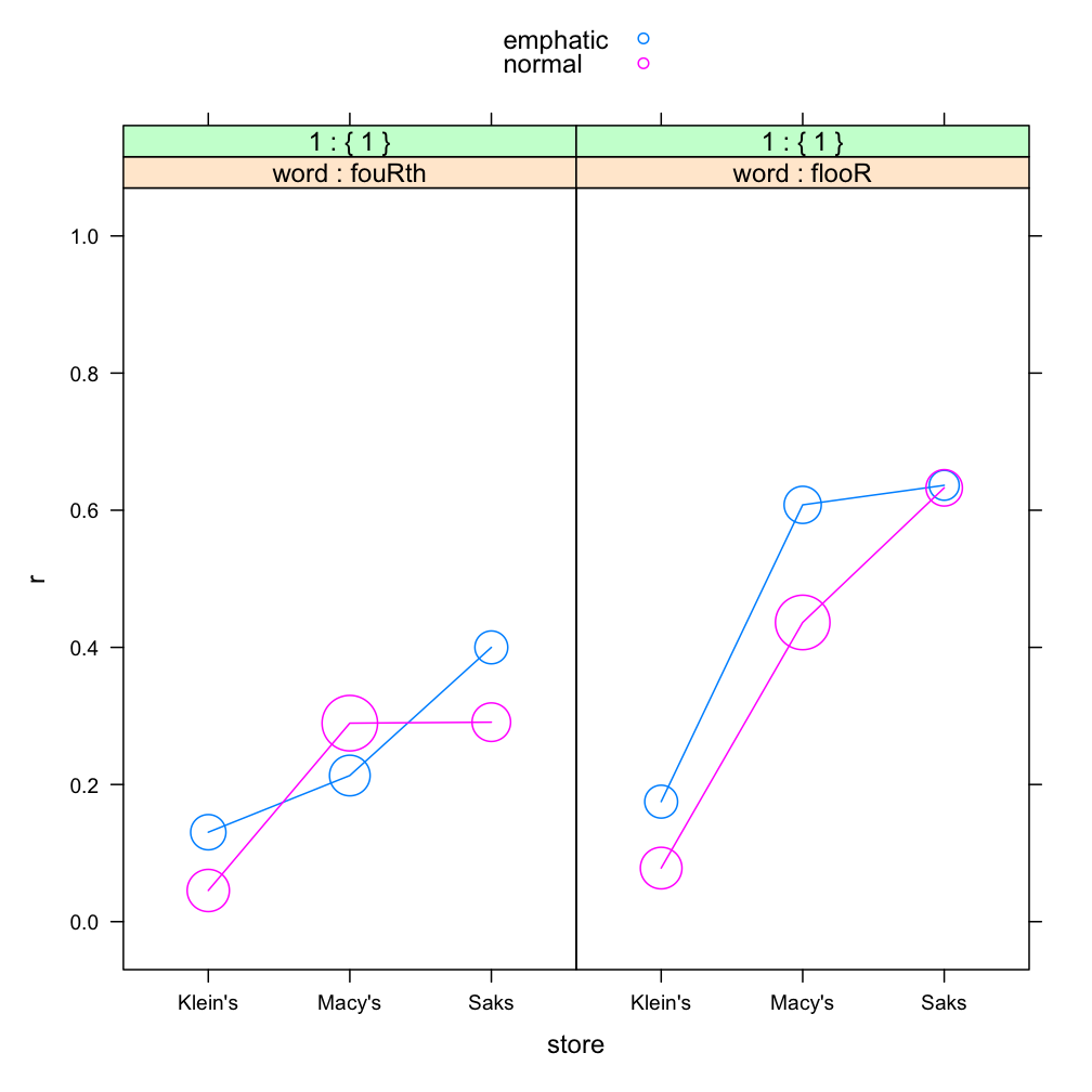
A plot like this is more informative than a cross-tabulation of the same data. The two main effects of store and word are clear. We can also see the somewhat inconsistent effect of emphasis, as emphatic pronunciations are usually more /r/-ful, but not in every case. We also note (as when we ran the crosstabs) that the slope associated with store appears decidedly steeper for the word floor than the word fourth. In part, this is due to the results being plotted on the probability scale, which makes changes in the middle of the range look bigger than changes towards the ends (constant change produces an S-shaped curve). Nevertheless, there is at least some interaction here, and since the model does not include an interaction term, this will contribute to a lack of model fit, as seen in the next custom scatterplot.
Choose variable for y-axis?
1: 5
Choose variable for x-axis?
1: 9
Separate (and color) data according to the values of which variable? (press Enter to skip)
1: 8
Also show data (in black) averaged over all values of word? (1-yes Enter-no)
1: [Enter]
Split data into horizontal panels according to which variable? (press Enter to skip)
1: [Enter]
Split data into vertical panels according to which variable? (press Enter to skip)
1: [Enter]
Type of points to plot? (raw points not recommended for binary data)
(0-no points 1-raw points Enter-mean points)
1: [Enter]
Scale points according to the number of observations?
(enter size factor between 0.1 and 10, or 0 to not scale points)
1: 0.5
Type of lines to plot (raw lines not recommended for binary data)?
0-no lines 1-raw lines Enter-mean lines)
1: 0
Add a reference line? (1-diagonal [y=x] 2-horizontal [y=0] Enter-none)
1: 1
Here we plot the model predictions on the x-axis, and the observed means for r on the y-axis. There are six points, because the model makes one prediction for every cell (3 values of store by 2 values of word). By coloring the points according to word this time, and adding a reference line at y=x (along which any perfect predictions would fall), we see that the overall fit of the model is good. The interaction between store and word is still noticeable: the leftmost blue dot, corresponding to floor at Klein's, is lower than it should be, while the rightmost dot for floor at Saks is higher than the predicted value; there is more social stratification for floor than the model predicts, and less for fourth. In the next section, we will explicitly test whether this interaction is significant, or at a chance level.

4. Testing for Interactions
Currently Rbrul does not handle interactions in a completely integrated way. However, if a model has been created (or loaded), a new option test interactions appears in the Modeling Menu. This tests each pair of model predictors for interactions. In this case:
MODELING MENU
...
11-test interactions
1: 11
Significance of interaction between store and word: p = 0.344
This tells us that the difference between the social stratification (store-related) slopes is actually not significantly different for the two words. That is, the observed interaction is not so large that it couldn't easily be due to chance. If the interaction were significant, new columns corresponding to the interaction would have been added to datafile, and the current model would have been updated to include the interaction. The predictions from that model would be accessible under Plotting, but the model details (factor weights, etc.) would not be. The smooth incorporation of interaction terms is a goal of future Rbrul development.
5. A Note on Knockouts
The Goldvarb software will not perform logistic regression if for any factor in any factor group, the data is invariant (i.e. the response proportion is 0% or 100%). I am not sure whether this restriction was originally computational or philosophical. Certainly it makes sense that if there truly are invariant contexts, they should be excluded from an analysis of variation. But when token numbers are small and probabilities are low or high, we will often observe cells that are unlikely to be "structurally" invariant, but do happen to be "knockouts".
Now it is true that it is difficult to accurately assess the response probability in a cell showing 0/10 or 10/10. But Goldvarb's reaction - that it not only cannot estimate the probability of such cells, but also will not estimate the probability of other cells of the same factor and, while it's at it, will not provide estimates for any other factor groups in the analysis - is certainly extreme.
For whatever reasons (meaning that I do not understand the reasons), the modern regression algorithms in glm and glmer do successfully handle the kind of data that would knock Goldvarb out. Once in a while, extreme invariance does cause the Rbrul regression to crash. Sometimes a NA will appear in the output. But usually a knockout factor will simply appear with a very low or very high coefficient and corresponding factor weight.
Computationally at least, this is an advance over Goldvarb, and we should not react suspiciously to the suggestion that computational statistics has made progress in the past 35 years or so. However, Guy (1988) argues that it is good practice to exclude invariant (and even near-invariant) contexts, no matter what. Rbrul allows this, but it also usually allows an analysis to be conducted on all of the available data, if desired.
6. About Mixed Models
Because Labov's department store data is so familiar, we might overlook that it has a very unusual structure for a sociolinguistic dataset. At each setting of the independent variables (say, floor with normal emphasis at Macy's) we have many observations of the dependent variable (110 in this case). Each of these observations comes from a different speaker. They are essentially independent. In sociolinguistic data derived from interviews, this is not the case: there, each speaker usually contributes many observations to the data, and it cannot be denied that tokens from the same speaker might be correlated with each other.
Because there are so many speakers, it is valid to make inferences about the populations (roughly, different social classes) that the speakers at the three stores represent. This would not be true if Labov had repeatedly queried only two or three people in each department store. In that case we would rightly wonder whether we were looking at a social class effect or "only" individual-speaker variation.
The opposite point can be made regarding the words in the study. Here we would be rather imprudent if we assumed that the behavior of fourth and floor (the latter word showed more /r/ than the former) directly generalized to all lexical items with word-internal and word-final postvocalic /r/, respectively. Believers in word-specific phonetics (Pierrehumbert 2002) might be especially skeptical. Readers of all theoretical persuasions will agree that in most sociolinguistic data, each phonological context is instantiated by a medium-sized number of words, not just one.
Coming from a kind of experiment, the department store tokens are also fairly well balanced across each independent variable, another feature which distinguishes this data from the majority of interview-based datasets. In real life, certain linguistic environments are less common than others and will always be underrepresented in the data.
In the last ten years, statistical methods have been developed which are appropriate for the kind of data sociolinguists usually work with: unbalanced data sets with internal correlations deriving from the tokens' being grouped by the two crossed factors of speaker and lexical item. Fitting regression models of this type is computationally difficult. Indeed, only since the release of Bates et al.'s lme4 package in 2006 has it been possible to fit mixed-effect models with crossed random effects to data with binary responses.
Psycholinguists have begun to take advantage of mixed models (see the Journal of Memory and Language, special issue on Emerging Data Analysis and Inferential Techniques). At least one contribution to sociolinguistics has done so as well (Jaeger & Staum 2005). One thinks of the 1970's, when the new techniques of logistic regression and VARBRUL sparked a quantitative revolution in sociolinguistics. We may stand today on the brink of a less profound, but still important advance. For while there is no denying the myriad results obtained over the years by fixed-effect variable rule methods, mixed-effect models promise better accuracy and reproducibility in many, if not most, sociolinguistically-relevant contexts.
To understand why this is so, it is helpful to make a three-way division among the predictors which may affect our response. This applies to both continuous and categorical predictors (and to both continuous and binary responses).
- External (between-speaker) predictors. For any given speaker, each of these takes only one value. For
example:
- age
- gender
- department store
- Internal (between-word) predictors. For any given word, each of these takes only one value. For example:
- following consonant (within the word, like in a study of vowel formants)
- lexical frequency
- whether post-vocalic /r/ is word-internal or final
- Other predictors. For these, the data for a single speaker, or a single word, can show more than one value.
For example:
- following environment (across words, like in a study of /t,d/-deletion)
- style
- emphasis
- by-speaker variation affects the significance estimates of external predictors
- by-word variation affects the significance estimates of internal predictors
Also, when the data is unbalanced or skewed (as it usually will be):
- by-speaker variation affects the coefficient estimates of external predictors
- by-word variation affects the coefficient estimates of internal predictors
The above points apply to both linear models (continuous response) and logistic models (binary response). In addition, in logistic models:
- by-speaker variation affects the coefficient estimates of internal and other predictors
- by-word variation affects the coefficient estimates of external and other predictors
With a binary response, the situation is different. Even if speakers all have the same size style effect -- for example, reading passage favors post-vocalic /r/ by a certain amount (in log-odds) over conversational speech -- if speakers differ in their overall rhoticity rate, then a fixed-effect model will underestimate the size of the style effect. In Goldvarb terms, if we did a separate run for each speaker's data, the factor weights for style would be the same in each; only the input probabilities would differ. But if we combined the data into a single analysis, the style factor weights would change, becoming less extreme and understating the true effect size.
This is because the log-odds difference between, say, 50% and 68% is roughly the same as that between 90% and 95%. So a speaker who style-shifts from 50% to 68% /r/ is exhibiting the same size effect as another speaker who shifts from 90% to 95%: 0.75 log-odds. But if these speakers' data were combined (assuming balanced token numbers) we would have an overall shift from 70% to 82%, which is only 0.64 log-odds.
Currently Rbrul can fit mixed-effect models with crossed random effects (e.g. for speaker and word), providing far more accurate estimates than Goldvarb, which would typically have to ignore these sources of variation.
A more advanced type of mixed-effect modeling involves not only random intercepts, as above, but random slopes. These capture the possibility that speakers (or words) might differ not just in their overall tendency regarding the response (different input probabilities), but also in their constraints regarding the predictors (different "grammars"). Further development of Rbrul will integrate random slopes, which can be thought of as interactions between fixed and random effects. The reader is referred to Pinheiro & Bates (2000) for further information about mixed models.
References
Guy, Gregory R. 1988. Advanced VARBRUL analysis. In Kathleen Ferrara et al. (eds.), Linguistic change and contact. Austin: University of Texas, Department of Linguistics. 124-136.
Labov, William. 1966. The social stratification of English in New York City. Washington DC: Center for Applied Linguistics.
Paolillo, John. 2002. Analyzing linguistic variation: statistical models and methods. Stanford CA: CSLI.
Pierrehumbert, Janet B. 2002. Word-specific phonetics. In Carlos Gussenhoven & Natasha Warner (eds.), Laboratory Phonology 7. Berlin: Mouton de Gruyter. 101-139.
Pinheiro, José C. and Douglas M. Bates. 2000. Mixed-effect models in S and S-PLUS. New York: Springer.
Jaeger, T. Florian and Laura Staum. 2005. That-omission beyond processing: stylistic and social effects. Paper presented at NWAV 34, New York.
Thank you for trying Rbrul.
Please report any bugs, unusual behavior, questions, suggestions for improvement, and/or topics for discussion to rbrul.list@gmail.com.
Return to DEJ Home Page